Back To The Basics
I’ve decided to compile the notes I’ve made over the course of my ML journey as a series of blog posts here on my website.
You can view other topics in this series by clicking on the ML NOTES category in the article header above.
Disclaimer
I’ve read through multiple sources; articles, documentation pages, research papers and textbooks, to compile my notes. I was looking to maximise my understanding of the concepts and, previously, never intended to share them with the world. So, I did not do a good job of documenting sources for reference later on.
I’ll leave references to source materials if I have them saved. Please note that I’m not claiming sole authorship of these blog posts; these are just my personal notes and I’m sharing them here in the hopes that they’ll be helpful to you in your own ML journey.
Take these articles as a starting point to comprehend the concepts. If you spot any mistakes or errors in these articles or have suggestions for improvement, please feel free to share your thoughts with me through my LinkedIn.
We’ll take a look at the Support Vector Machine + understand the kernel trick in this post.
Support Vector Machine
Support vector machines are a type of supervised learning algorithms mainly used for classification.
Support vector machines divide the input space into “class areas” using hyperplane(s) and then classify samples based on the side of the hyperplane they fall to.
The SVM algorithm tries to find the optimal hyperplane separating the two classes by maximizing the distance of the hyperplane from both classes; that is draw the separating hyperplane in between the classes such that it is as far away as possible from both the classes so it can achieve the best classification outcome.
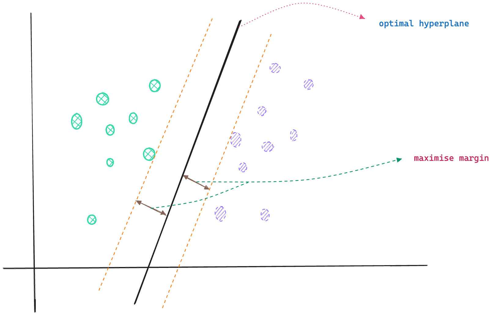
Certain data points are hard to classify as they fall very close to the decision boundary. These data points are called support vectors, and the SVM algorithm makes use of these support vectors to draw the optimal hyperplane such that the distance between the hyperplane and the support vectors (from both classes) is maximised.
The choice of the support vectors influences the optimal hyperplane and its orientation in space.
SVM classifiers work well for linearly separable classes by setting up the optimal hyperplane using support vectors.
Regularization Parameter C
The width of the margin around the separating hyperplane is governed by C, known as the regularization parameter, influencing the model’s ability to generalise well on unseen (test) data.
C is inversely related to the width of the margin; a small C value results in a wider margin, and conversely, a larger C value results in a narrower margin.
Small C, Wider Margin
A small value for C results in a wider margin, a configuration useful for scenarios where you want to improve the model’s generalization ability at the cost of (some) training accuracy.
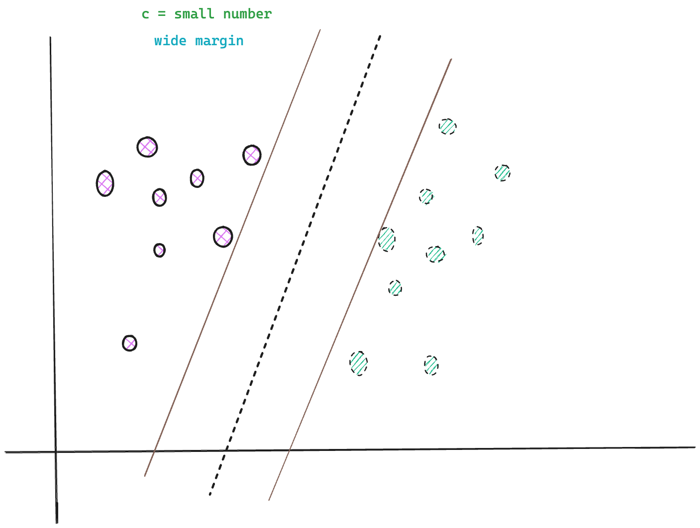
Having a wider margin could result in misclassification of data points near the decision boundary, leading to a lower training accuracy. However, a wider margin allows the model to generalise well and reduces the risk of overfitting.
This configuration is appropriate when the data has a lot of outliers or noisy samples. In this case, a small C value allows for a wide margin which ignores the outliers, and because the model isn’t chasing noise, it performs better on new, unseen data.
However, you must still be careful not to set the C value to a very small number as that can result in too wide a margin, and underfitting, where the model fails to learn the underlying patterns in the data.
Large C, Narrow Margin
Setting the C value to a large number results in a narrower margin which is useful when you want to improve the model’s training accuracy. A large C value penalises misclassifications on the training data.
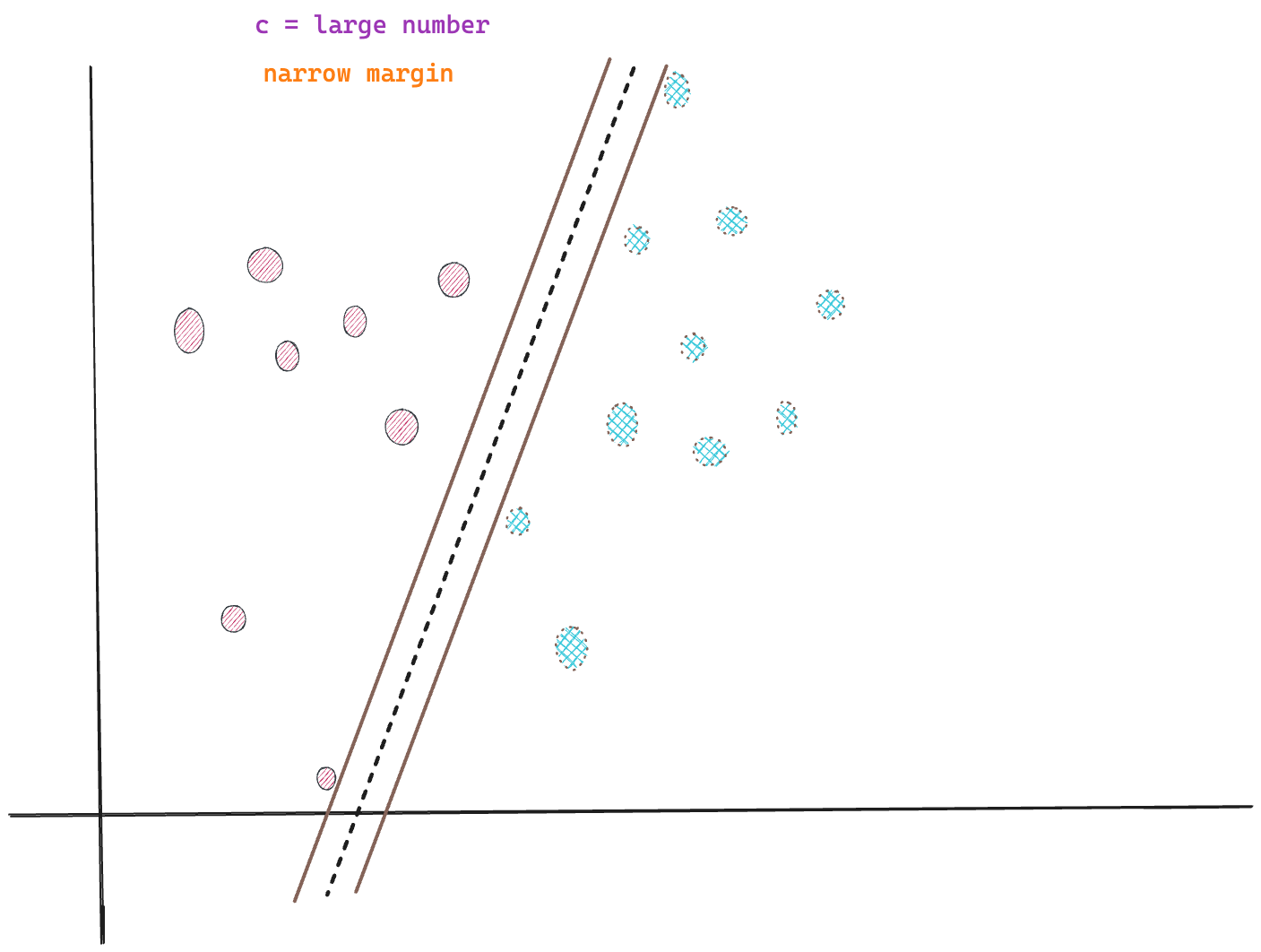
This configuration is suitable for scenarios where the dataset has less outliers or noisy samples.
However, once again, care has to be taken when setting the value of C, as too high of a value can result in an extremely rigid and narrow margin, overfitting; where the model is tuned too accurately to the training data, including the noise samples, and fails to perform well on the test data.
Couple of techniques that can help find a near-optimal value of C include grid search, bayesian optimization etc.
Kernel Trick
When the data are not linearly separable, then it is no longer possible to use linear structures to separate the classes. However, the SVM model can still be used to achieve classification on non-linear data through the use of the kernel trick.
The kernel trick involves mapping data to a higher dimensional space from the original dimension in the hopes that a separation between the classes is exposed in the new, higher dimension.
Transforming the data from the original feature space to a higher-dimensional space by applying a non-linear transformation function is a non-trivial operation, especially if the original feature dimension of the data is already high.
If you do not use the kernel trick, the manual way would first involve transforming all data points in the dataset to a higher-dimensional space, then computing the optimal hyperplane to divide the classes in this new, high-dimensional space.
Using the kernel trick eliminates the need for the explicit and expensive transformation operation. The kernel function (depending on the type of the kernel function used) calculates a measure of similarity between a pair of vectors (representing a pair of data points) in the original feature space. The process is then repeated for all other data point pairs.
The kernel function, therefore, allows us to figure out which data points are similar, or lie closer to each other, in the higher-dimensional space without actually transforming the datapoints to the higher-dimensional space
The choice of kernel determines the type of patterns the SVM is good at capturing.
Types of Kernel functions
1. Linear
The linear kernel function helps find a flat decision boundary and is not good for separating classes for non-linear data. The linear function is essentially a regular dot product between the data point vectors.
\[K(x, y) = \mathbf{x}^T \mathbf{y}\]
- \(\mathbf{x}\) and \(\mathbf{y}\) are matrices representing the coordinates of data points in the original dimensional space
- \(\mathbf{x}^T\) is the transpose of the \(\mathbf{x}\) matrix.
When you set the kernel parameter to “linear” in scikit-learn’s SVC class, the kernel trick is not applied.
2. Polynomial
The polynomial kernel function considers non-linear interactions between the data points. This helps it create curved boundaries capable of separating classes in non-linear data.
\[K(x, y) = (\mathbf{x}^T \mathbf{y} + c)^ d\]
introduces non-linearity, \(c\) is a constant, \(d\) is the degree of the polynomial function.
3. Radial Basis Function (RBF)
In machine learning, the Radial Basis Function (RBF), also known as the Gaussian Kernel, is a popular kernel function used in various kernelized learning algorithms. The formula for the Radial Basis Function is:
\[ K(x, y) = \exp\left(-\frac{||\mathbf{x} - \mathbf{y}||^2}{2\sigma^2}\right) \]
- \(||x - y||²\) represents the squared Euclidean distance between \(\mathbf{x}\) and \(\mathbf{y}\)
- \(\gamma ={\tfrac {1}{2\sigma ^{2}}}\) is a free parameter that needs to be set manually
💡 RBF Intuition
The \(||\mathbf{x} - \mathbf{y}||²\) represents the squared Euclidean distance between the data points \(\mathbf{x}\) and \(\mathbf{y}\). The overall effect of this function is to create a measure of similarity between \(\mathbf{x}\) and \(\mathbf{y}\), which decreases as the distance between them increases.
If the distance between the data points is large, then both the squaring operation and the exponential operation will blow up the distance. If you consider the right hand side component in its entirety, you will find that its value decreases when the distance in the numerator increases and vice versa.
The right hand side component is nothing but a measure of similarity and it ranges from 0 to 1. So, the output of the RBF for 2 datapoints gives us a directly interpretable measure of similarity between the data points.
The RBF kernel effectively computes a measure of similarity between the data points as if they’d already been mapped to the higher dimensional space without actually doing the transformation.
It expands (or reduces) the distance between non-similar (or similar) data points, creating sparse areas in between classes. The SVM algorithm is then able to draw the separating hyperplane between the classes in these areas of sparsity.
Also, it seems to me that the RBF kernel function calculates a sort of “tiny hyperplane” between each pair of data points; and repeats this exercise for all the datapoints.
So, when you connect all the tiny hyperplanes together you end up with a curved hyperplane that is able to zigzag and weave in through the space in all sorts of manner; essentially achieving good separation even for non-linearly separable classes.
This ability to use similarity allows the RBF kernel to create sophisticated decision boundaries, even when dealing with complex and non-linearly separable data.
Guidelines for working with SVMs
Below are some points to keep in mind when working with an SVM model:
1. Non-Linear data: From what we’ve seen so far, SVMs (+ kernel functions) can be used for data which is not linearly separable. So, if you find your data has non-linear relationships, you might want to start experimenting with the SVM algorithm and the different kernel functions.
2. High-Dimensional Spaces: SVM (with no kernel trick) can perform better in high-dimensional spaces (where the number of features is much greater than the number of observations) due to its reliance on support vectors, rather than on dimensionality. However, as the number of features increases, the computational complexity of training the SVM algorithm also increases.
3. Small to Medium Dataset: SVM can be more effective for small to medium complex datasets (especially if they have a lot of sparse values) since its optimization doesn’t depend as heavily on the number of data points, focusing instead on the support vectors. However, SVMs with kernel optimizations do not scale well to large numbers of training samples, or large number of features in the input space.
4. Sensitivity to Outliers/Robustness: If your data has outliers or noise, SVM might be more robust since it focuses on the support vectors closest to the decision boundary.
5. Model Complexity + Training time: SVM can be computationally more intensive, especially with large datasets and when using complex kernel functions. The training time can also be considerably longer for large feature spaces.
6. Global Optima: SVMs tend to find the global optima for a given task, and avoid the problem of getting stuck in the local minima. Moreover, SVMs also have a small number of hyperparameters, the kernel function and the regularization parameter C. These properties might be more attractive over other models such as neural networks.
7. Interpretability: SVM models, especially with non-linear kernels, are less interpretable, making it harder to understand the relationship between input features and the predictions.
Thanks for reading! Hope you’ve found this post helpful, and as always, pop in occasionally to this space to read more on machine learning.
References
- An Idiot’s guide to Support vector machines (SVMs) by Professor R. Berwick
- How SVM Works
- Radial basis function kernel